NCI-CPTAC DREAM Proteogenomics Challenge: Ardigen’s Second Place Solution

From this article, you’ll learn:

1. What the Dream Challenges are about,
2. How the NCO-CPTAC Dream-Proteogenomics Challenge looked like from our perspective,
3. What was the first stage of the challenge,
4. How the second challenge went through,
5. How we shaped our model architecture,
6. What was the drive behind choosing the best starting model,
7. How the sub-challenges model details, such as variables and ensembling, was shaped like,
8. Conclusions

About DREAM Challenges – Biology Experts United

Since 2006, DREAM Challenges have been posing fundamental questions about systems biology and translational medicine [1]. Unlike the mainstream machine learning competitions on Kaggle [2], the DREAM Challenges do not end with establishing the final leaderboard of participants. Instead, there is usually a follow-up community phase, in which the top teams combine and improve their models and use them to gain scientific insights into the addressed biological problem. Later, prestigious scientific journals publish the final results [3].

NCI-CPTAC DREAM-Proteogenomics Challenge Through the Lenses of Ardigen Experts

The NCI-CPTAC DREAM-Proteogenomics Challenge [4] focused on predicting the protein concentrations in cancer tissues. Characterization and analyses of alterations in the proteome can shed more light on cancer biology and may improve the development of biomarkers and therapeutics. As measuring proteomic data is both difficult and expensive, the challenge objective was to develop machine learning models for predicting such information based on genomic and transcriptomic data.

The challenge consisted of three sub-challenges. Ardigen’s team took part in the second and third, securing the fifth and second place, respectively.

• → For sub-challenge 2, their objective was to predict protein abundances based on genomic – that is, copy number alterations and CNA – and transcriptomic – meaning mRNA expressions.
• → Sub-challenge 3 included both these goals with the addition of phosphoprotein data.

Our team’s solution applied directly to the sub-challenge 2. Therefore, now we will dive into its details while highlighting this segment.

About Proteogenomics

Proteogenomics is a multi-omics research approach that sheds new light on cancer development. Integrating genomic, transcriptomic, and proteomic information can lead to a deeper understanding of the complex processes related to cancer and the development of novel biomarkers and therapeutics.

NCI-CPTAC Dream Proteogenomics Challenge – the Data and the Task

The challenge data provided by the Clinical Proteomic Tumor Analysis Consortium (CPTAC) [5] measured for ovarian and breast cancer. The proteomic data was measured by two laboratories: John Hopkins University (JHU) and Pacific Northwest National Lab (PNNL) [6]. The median Pearson correlation of paired protein measurements from the same sample, measured in the two laboratories, was 0.69. This result already shows how difficult it is to measure the proteome.
The challenge dataset was high-dimensional with around 100 input observations – in other words, samples – and typically from 10,000 to 35,000 features. These include:

1. CNAs,
2. gene expressions,
3. protein abundances [4].

In the 2 and 3 sub-challenges, the task was to predict around 1,000-15,000 target variables. The metrics used to measure the performance was the average Pearson correlation between predicted and measured (phospho)protein abundances.

The Ardigen Team Composition

The Ardigen’s team consisted of four experts who repeatedly discussed the model development strategy.

• → Jan Kaczmarczyk proposed the general architecture of the models and implemented them,
• → Łukasz Maziarka suggested vital improvements in the models,
• → Piotr Stępniak provided bioinformatics support,
• → Michał Warchoł guided model design.

NCI-CPTAC DREAM-Proteogenomics Challenge – the First Stage of Model Development

At the beginning of the challenge, we tested standard approaches to high-dimensional data. These include the lasso and relaxed lasso methods [7] and a random forest model with feature elimination (e.g. leaving the 100 key features after the first fit). The cross-validation scores of these methods were slightly below the 0.38 mean Spearman’s correlation between mRNA and protein abundances observed for ovarian cancer [6].

However, when submitted to the challenge and evaluated on a prospective dataset, the scores of these models were much lower. After submitting a baseline model built on a single variable (mRNA or – in its absence – the variable with the highest correlation to the target protein) and observing that it scored 0.38 (in sub-challenge 2), we have decided to develop models using the forward feature selection and restricting ourselves to a small number of predictors.

Dream Challenges – Ardigen’s Second Stage of Model Development

In the second step, we tested models with engineered features – aggregated variables relating to gene sets provided in the ovarian cancer study [6] and those from the MSigDB Collections [8]. These models performed well locally – that is, on a holdout set. However, they gave significantly lower scores (0.41 in sub-challenge 2) when submitted to the challenge.

We concluded that generalization is an issue in this competition and that batch effects play a role. Moreover, the generalization properties of developed models depend significantly on the type of variables on which the models are built. We addressed this issue explicitly in our final solution by using an auxiliary model to predict how well-selected models generalize: we trained models (on one or two variables) using PNNL data. We tested them on JHU data of the ovarian cancer dataset in sub-challenge 2.

These models enabled us to predict how well the starting model in our forward feature selection algorithm will generalize (in other words – how robust it is against batch effects) and select the best one among a few such starting models. Afterward, we added variables to the chosen starting model in a standard manner – that is, via forward feature selection.

Our final models scored:

1. 0.46 (for ovarian cancer) and 0.42 (for breast cancer) in sub-challenge 2,
2. 0.29 (for ovarian cancer) and 0.36 (for breast cancer) in sub-challenge 3.

These scores gave us fifth place in sub-challenge 2 and second place in sub-challenge 3.

Our Model Architecture

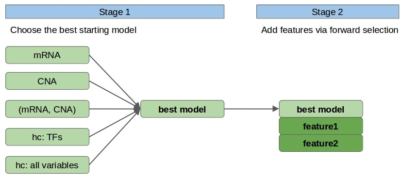
During the challenge, we used a two-stage hierarchical forward feature selection algorithm. The first stage focuses on variables showing good generalization properties as determined by an auxiliary model. We used its residuals in the second stage by fitting them into a separate model.

Model Architecture: Stage One

In stage 1, we choose the single, ‘most promising’ model among models built using linear regression on the following sets of 1-2 variables: mRNA, CNA (mRNA, CNA), hc: TFs, hc: all. Here, mRNA and CNA denote the features relating to the considered protein (i.e. with the same GeneID), the only set with two variables is (mRNA and CNA), and by hc, we mean the variable with the highest correlation to the target variable from a given set of variables.

In particular hc: TFs denotes the variable chosen among mRNA and CNA of human transcription factors (TFs) [9], whereas hc: all variables denotes the variable chosen among all variables. From the hc: TFs and hc: all candidate feature sets we remove mRNA and CNA relating to the considered protein. We use TFs as a separate set of variables because limiting ourselves to a relevant subset of the original features should decrease noise.

Model Architecture: Stage Two

In stage 2, we fit a separate model to the residuals of the model obtained in stage 1. To this end, we use a forward feature selection procedure. For the early-stopping criterion, we consider the cross-validation (CV) score change when adding a variable. We follow a customized cross-validation procedure with five folds and a holdout set. The holdout set (with ~20% of data) is used to obtain a more realistic (not overfit) estimation of model performance.

Additionally, we impose a barrier, b, for the enlargement of the model by variable(s) being added. If the considered variable(s) does not improve the CV score by at least b = 0.06 (for ovarian cancer) or b = 0.07 (for breast cancer) it is rejected and the procedure stops. The values of b = 0.06, 0.07 were determined by optimizing for the holdout set score. Note that the feature with the highest correlation to the residuals of the current model is chosen per train-test split in the cross-validation procedure and can even be a different feature for each split.

Choosing the Best Starting Model

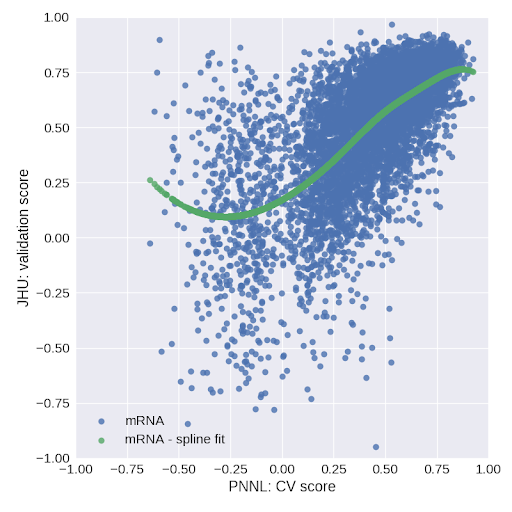
In stage 1 of our algorithm, we choose the best model among several candidate models. Typically the cross-validation score (or holdout set score) can be used for such a task. However, as generalization was an issue in this challenge, we used an auxiliary model for this purpose. Namely, for all proteins in the ovarian dataset of sub-challenge 2, we train the models considered in stage 1 on the PNNL data and test them on the JHU data (cf. Fig. 2).

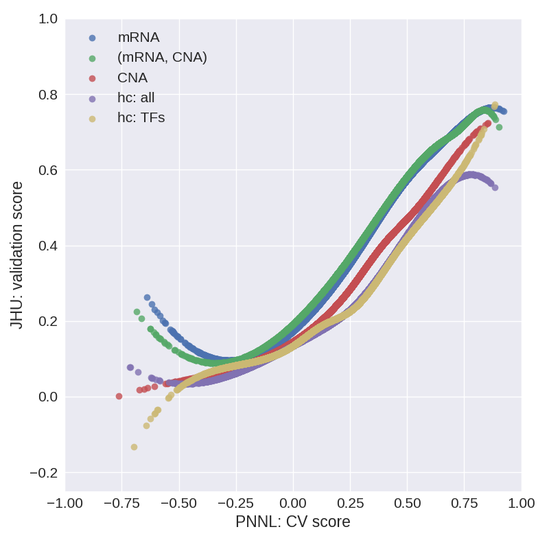
The relation between the CV score on PNNL data and the validation score on JHU data is a measure of how well selected models generalize. We then fit a cubic spline with 4 knots (extrapolated linearly above the fourth knot due to oscillatory behavior in this regime) to the (CV score, validation score) data and use it for predicting the validation score of selected models in stage 1. Figure 3 shows cubic splines obtained in this manner for the models considered in stage 1.

We observe that models built on mRNA or (mRNA, CNA) show the best generalization properties, followed by models built on CNA and then by the hc: all and hc: TFs models. Explicitly, in stage 1 we take the cross-validation score of selected models as a predictor in the auxiliary model and, thereby, we predict the validation score. The predicted validation score is then used for selecting the best model.

Sub-Challenges Model Details: Transformations of Variables and Ensembling

For all our models in sub-challenge 2 we use unregularized linear regression, whereas in sub-challenge 3 we use least angle regression (LARS) implemented in the LarsCV class in the sklearn package in Python.

For imputation we use the mean imputation. We also tested several transformations on the predictors, of which X→log(X+B ) and (X, Y )→(X, 2Y ) are included in our final ensemble of models. As a final solution, we use ensemble of models over different fold splits and – in sub-challenge 2 – with the above transformations of variables.

In our final submission, we use an ensemble of 15-65 models per (phospho)protein for both the ovarian and breast cancer datasets. The models within an ensemble differ by the splitting to train-test sets of the cross-validation procedure. We use the 5 models trained per train/test splits instead of retraining the model on the entire data. In sub-challenge 2, we also determine our choice by the variable transformations used. The gain from ensembling is around 0.01 in sub-challenge 2 and 0.04 in sub-challenge 3, as determined on a holdout set.

NCI-CPTAC DREAM-Proteogenomics Challenge – Conclusions

In an early stage of the challenge we observed that the submitted models differed significantly in how well they generalized to the online-evaluation data. To address the issue of model generalization we used high-bias models (linear regression and least angle regression) augmented with auxiliary models to predict generalization properties of selected starting models. Construction of such auxiliary models was possible because sub-challenge 2 contained data measured by two laboratories, which enabled us to quantify generalization of selected models. In sub-challenge 2 we also used transformations of variables. In both sub-challenges we used ensembling; however, the improvement it provides is much higher in sub-challenge 3.

The Outlook

As our solution scored with the second place in sub-challenge 3, we were invited to the community phase, in which we worked on a joint improved solution with the winning team: Hongyang Li and Yuanfang Guan from the University of Michigan. As a result, the performance of the models was significantly improved (from the mean Pearson correlation of 0.33 to 0.37 for the ovarian cancer, and from 0.42 to 0.48 for the breast cancer). At the moment the organizers of the challenge and the top teams of sub-challenges 2 and 3 are finalizing a manuscript on the results of the sub-challenges, which is to be submitted to Nature Methods. More details on the collaboration can be found in [10].

Works Cited:

[1] dreamchallenges.org

[2] www.kaggle.com

[3] dreamchallenges.org/publications

[4] NCI-CPTAC DREAM Proteogenomics Challenge, www.synapse.org/#!Synapse:syn8228304/wiki/413428

[5] Clinical Proteomic Tumor Analysis Consortium (CPTAC), proteomics.cancer.gov/programs/cptac

[6] Zhang H, Liu T, Zhang Z, Payne SH, Zhang B, McDermott JE, et al., Integrated Proteogenomic Characterization of Human High-Grade Serous Ovarian Cancer, Cell 2016;166: 755–765. doi.org/doi:10.1016/j.cell.2016.05.069

[7] Hastie T, Tibshirani T, Tibshirani RJ, Extended Comparisons of Best Subset Selection, Forward Stepwise Selection, and the Lasso, https://arxiv.org/abs/1707.08692

[8] MSigDB Collections, software.broadinstitute.org/gsea/msigdb/collections.jsp

[9] A resource for Human, Mouse and Rat Transcription Factors, www.tfcheckpoint.org/index.php/introduction

[10] Best Performers Announced for the NCI-CPTAC DREAM Proteogenomics Computational Challenge, proteomics.cancer.gov/news_and_announcements/best-performers-announced-nci-cptac-dream-proteogenomics-computational