Conformal Prediction in Classification

Introduction

When developing machine learning models to solve your problem, the standard way of testing their performance is to measure it on a held-out test subset. This way, you obtain a notion of how well your model fits the data. Unfortunately, you have no idea about the certainty of the model when it comes to individual predictions. But what if we reversed that order and instead, we began with setting a level of confidence we want our model to conform to? Then, our model would be able to predict if individual predictions are reliable or not – assuming the given confidence level.

Conformal Prediction does exactly that. It quantifies the uncertainty of each prediction separately. What is great about this framework is that it is model agnostic – it works with any machine learning algorithm.

Most machine learning algorithms predict point estimates. Conformal Prediction, however, returns set-valued predictions. In the case of classification, it outputs a set of labels. For example, the ImageNet (ILSVRC subset) contains 1000 classes out of which 90 are dog breeds. For some input images, our Conformal Prediction could output a single class as certain with given confidence. For another input, we could get a set of 200 various labels, while another input could output a set of 50 dog breed labels. In extreme cases, we could end up with a set of all labels or an empty set. The algorithm guarantees that the true label is present in the prediction set with the given probability (confidence).

Figure 1.
Conformal Prediction output example. Ground truth label in red.

How do you interpret such results? It may not be straightforward at times and it may depend on the task at hand. When we receive a set with only a single label, the model is certain about its prediction. If the CP outputs a set of 5 dog breeds and we don’t care that much about what dog breed is present in the picture, we can state with quite high confidence that the image contains a dog. If the algorithm outputs a set of 500 classes, we could say that it is rather unsure of its predictions and perhaps we should not act on it.

There are two Conformal Prediction settings: online and inductive. The former analyzes the inputs one by one and each successive prediction depends on the previous one. The latter does not require consecutive execution and hence it is less computationally expensive. In this blogpost, we will focus entirely on the inductive setting.

There exist multiple extensions to the basic variant of the algorithm. Here, we focus on Mondrian Conformal Prediction. I picked it because it guarantees that the confidence levels are met for each class independently.

Requirements

Let’s get a little bit more specific. To run Conformal Prediction we will need:

1. Predictive model
2. Calibration set
3. Non-conformity measure

Model could be any classifier, for example a ResNet to match our ImageNet example.

Calibration set has to contain pairs of input and label that come from the same distribution as the training set. However, these examples cannot be seen by during training.

The non-conformity measure quantifies how “strange” a label is for a given instance . A commonly used function is

where is the softmax output of the model for a given class here indicates that it might be interpreted as the probability of the model assigning this class). There are no formal requirements for the non-conformity measure. It could even be a random number generator, but don’t expect great results in such a case.

Mondrian Conformal Prediction algorithm

Our dataset consists of pairs of input data and label (e.g. is an image and is one of 1000 aforementioned ImageNet classes). Apart from the regular train/validation/test split, we also need to make room for an extra calibration set. All four subsets must be disjoint. In the case of ImageNet, where the training set is rather large, a straightforward solution is to create the calibration set from a fraction of the training set. We train the model using the new split. Now we’re ready for the first step – calibration:

1. Compute nonconformity scores on the calibration set (n data points):

2.  Pick the confidence level

3. Iterate over all labels and find   – nonconformity score at c -th percentile for label  L

4. Store the thresholds – they will be used during inference.

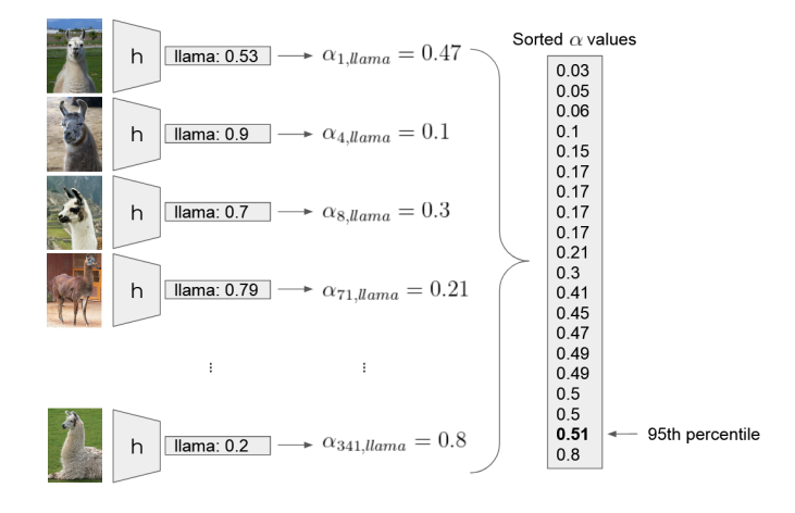
Calibration example of the “llama” label. Let’s assume there are 20 images with this label in the calibration set. We input each image into the model , fetch the softmax output for the “llama” class  and compute the nonconformity score .  We collect all the nonconformity scores and find the 95th percentile .

During inference, we input a new image . We iterate over all labels and exclude label  L if nonconformity score is higher than threshold . Otherwise we keep the label. For example:

We might end up with a set of labels

Again, how to interpret such a result? If our task is to state if there is a fish in the image, then we’re rather certain that it’s absent. But, if we would like to distinguish wigs from burritos, we can say that our model is not certain about that.

The procedure guarantees that

for each class separately – expected probability of the correct label being included in the output set is c.

Evaluation

The error level is defined by the user, so it cannot be used to measure the quality of predictions. Instead, we can look at the size of the output prediction set, e.g. the average number of output labels.

We can also measure efficiency. The algorithm is efficient when the output prediction set is relatively small and therefore informative. We can define efficiency as the number of predictions with only one label divided by the number of all predictions.

Yet another measure is called validity. We can define it as a fraction of the predictions with only one label that were predicted correctly.

Summary

This blog post sheds some light on how to apply Mondrian Conformal Prediction to a classification problem in the inductive setting. Key take-home messages:

1. Conformal Prediction quantifies uncertainty of each prediction separately.
2. It’s flexible – any predictive model can be applied.
3. It outputs set-valued predictions instead of point estimates.
4. It provides error rate guarantees.

References

Original book that introduced the method:

Vovk, Vladimir & Gammerman, Alex & Shafer, Glenn. (2005). Algorithmic Learning in a Random World.

This blog post relies on:

https://www.youtube.com/watch?v=eXU-64dwHmA