
Is the machine learning model good enough?
Simply applying the machine learning (ML) model to answer biological questions is only the beginning of the story. If we want to use the model to stratify new patients, or publish our findings, we need to be able to estimate how effective the model is.
The key measurable quality of a model is how well it performs on unseen data, which we obviously have no access to. Thankfully, we can reliably approximate our model’s performance by using a method called cross validation (CV).
CV allows us to judge a model in objective terms and determines if what it learned is an actual biological signal or just some random noise, which would not generalize well to new unseen cases. If the model copes well in CV it means we can trust its predictions and proceed to interpret what it had learned.
In the simplest case, CV is performed by setting some of the original data aside, letting the model train on the remaining samples and validating its predictions on the data we left out (called a split into train and test data). This, however, leaves us susceptible to a stroke of good (or bad!) luck—we may have selected samples easiest to predict for the test set, so the process resulted in an overly optimistic performance estimate?
Enter the cross validation
CV was created to avoid such a bias: it repeatedly splits the data, training and testing the models on each data split independently. This way, instead of just a single estimate we get the whole set of numbers: complete statistics of estimates, from which we can derive a more thorough understanding of the model’s performance.
There are multiple ways of implementing cross validation, depending on data availability, type of predicted values (e.g. categorical or continuous), and available computational power. By far, the most common implementation is a repeated k-fold cross validation, but other prominent examples include out-of-bag bootstrap and leave-one-out CV.
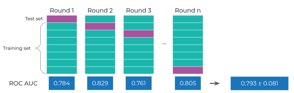
Figure 1. The cross-validation approach for model validation. The data is first divided into folds (the purple and green blocks). In a single CV round, we designate one block as the test set (purple) and the train set (green), train the model on the train set and evaluate it on the test set yielding a single score value (in blue, at the bottom, we used ROC AUC as an example). We repeat the process by selecting a different test fold each time until all folds are used as a test yielding a distribution of model performance scores.
For the k-fold CV (Figure 1), we split the data into folds (roughly equally-sized chunks, where k is the number of chunks). We then go through the folds one-by-one, using the selected fold as the test set and the remaining ones as the train set. This way, we guarantee that all the samples will become a part of the test set and diminish the risk of choosing a lucky test set. To get an even more robust estimate, it is recommended to use a repeated k-fold CV, which randomly splits the data into a fold multiple times. The more repetitions, the more robust the results and the risk of a stroke of luck is considerably limited. [2, 3].
Flavors of cross validation
So far, we described how to apply CV in a case where we had one data set, that is, an intra-cohort CV. This type of validation is always available as we always have a data set when applying ML. However, the estimates derived this way hold only if the upcoming data is expected to be very similar to the data set at hand. Imagine analyzing data from a not well-known study conducted in a distant country on a group of elderly women. Even if we rigorously apply CV on this data the intra-cohort estimates will only be of limited use if we plan to deploy a model to stratify a group of young men in your country.
If, however, we have access to other data sets, we can implement a more thorough evaluation scheme. We can train the models on patients from one data set and use the other data set to test what the model has learnt. This way, we will see if the model picked up some signal that can be generalized to another population. This can also be done in the other direction by swapping the data sets. The process of training and testing the model on different data sets is often called a cross-cohort (or cross-group) CV [3, 4, 5], see Figure 2.
Intra- and cross-cohort CV results can tell you a lot about the data at hand. For example, if a model does well intra-cohort but not cross-cohort, it means that it is likely picking up on effects specific to each of the populations, so deriving broad general statements based on these data sets may be risky. However, if both intra- and cross-cohort CV results are good, you should be safe to claim that you are onto something.
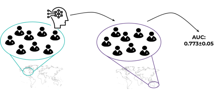
Figure 2. The general idea behind a cross-cohort validation: a model is trained on one cohort and evaluated on a completely different cohort (here a geographically different one). This way we can check if the model captures some actual biological effect and is not restricted to a single population.
Going even further, if we have more data sets at hand we can employ a leave-one-dataset-out CV (LODO). As the name suggests, we look at how the model performs when tested on a given data set but trained on all the others. This scenario is useful to see if merging multiple data sets leads to improved performance and generalizability by allowing an algorithm to learn more general patterns [1].
Combining all of the above techniques leads to a comprehensive set of CV results, by which we can judge our ML models and claim that what we found is sound. Of course, having multiple data sets is a luxury not every research problem can afford and often we have to make do with what we have and use intra-cohort validation only.
Good practices are key
Although CV and its variants may seem trivial to apply – just split the data, fit the models and evaluate them – there are certain things that you should keep in mind before you start using it.
One particular example of CV misuse, prevalent in scientific papers, is feature selection outside of the CV process. The features (e.g. abundance of specific taxa) are first analyzed with statistical tests to identify the ones most related to the predicted variable (e.g. by a p-value cutoff). Then, a CV procedure is employed to check the model’s performance on these selected features only, instead of the complete set. This, however is a mistake, because the features were selected based on all data, including the samples that will become a test set. We could say that the test set leaks information into the model as it contributes to the selection of the features for the ML model (hence the name “data leak” in ML terminology). The model will typically perform better with such leaked knowledge than without it, so even though we apply CV, it will lead to an overestimated performance value. The remedy is to integrate the feature selection into the CV process, and perform feature selection on the train set only, which eliminates the data leak. The rule of thumb is, the earlier in your analysis you employ CV, the better.
Also, if you use CV for a classification problem you should split your data in a stratified way, so that the various classes are proportionally represented in the train and test sets. This is not trivial in some extremely small data sets and in cases of highly imbalanced data. In some scenarios, you may even have to resort to data augmentation.
The number of splits is also something that should be carefully considered: the more splits, the larger the train set, so the model can learn more, but it also means a smaller test set, leading to perhaps higher, but more widely varying performance estimates (higher variance).
And we have not even mentioned the nested CV yet, which allows you to, among others, safely optimize model hyperparameters without risking biased outcomes. All in all, there is much more to the CV process than meets the eye: CV is easy to learn but hard to master and often has to be fine-tuned to the data at hand.
What else is cross-validation good for?
The usefulness of CV does not end at faithfully evaluating model performance. You can use the randomized train/test splits to evaluate any property of your model. Taking linear regression as an example: fitting the model once yields only a single weight value. However, if you fit the same model to various CV train sets, you will get a whole spectrum of weight values, which you can use to identify the most confident weights. This is most commonly done with a bootstrap variant of CV.
Another, more obvious, application of CV is model comparison. If you can not decide what is better: a random forest or a logistic regression, you can pick one based on their CV scores. But then you should remember to use exactly the same CV splits for both.
Finishing thoughts
Cross validation leads to accurate estimates of how your machine learning model will perform on new data. This information is crucial for selecting the right model or even determining if there is any signal in the data. Although it is a powerful tool, you should not apply it blindly without first considering the specificity of the data at hand and selecting an adequate variant. Remember that whichever variant you decide on, you should always state your choice when presenting your findings, which will make it easier for others to compare their results with yours.
In our previous blog post, we pointed out that machine learning has not yet fully taken hold in the microbiome literature. Cross validation is often similarly neglected, sometimes models are presented without any validation at all, sometimes there is a data leak biasing the results of CV.
At Ardigen, we uphold the highest standards when using CV, which gives us and our clients the confidence to tackle the most challenging problems. Fine tuning the cross-validation process keeping the clients in the loop, informing them about possible choices and accompanying tradeoffs is a part of every project. This transparency leads to higher confidence in the results and allows each partner to fully understand the delivered results and their meaning to their business.