
The integration of AI in medical imaging is revolutionizing the field of radiology, particularly in the analysis of brain MRI scans. By utilizing modern AI techniques, radiologists can access innovative tools that significantly advance the diagnosis of neurodegenerative diseases and completely transform the way we interpret MRI data. See the changes that will redefine the landscape of medical imaging.
Leveraging AI in medical imaging has opened fresh perspectives in the analysis of brain MRI scans. This article explores how modern AI techniques enhance radiology practices, offering a groundbreaking approach to diagnosing neurodegenerative diseases and redefining our methods of comparing MRI data.
The Transformative Role of MRI Scans in Neurology
MRI scans play a crucial role in both diagnostics and clinical trials. They help assess a patient’s health during the treatment of various neurodegenerative diseases, including Alzheimer’s disease, frontotemporal dementia (FTD), multiple sclerosis, Huntington’s disease, Amyotrophic lateral sclerosis (ALS), and others [1].
Using MRI scans, we can gain insights into how these diseases affect the brain, as demonstrated in the following example [2]:
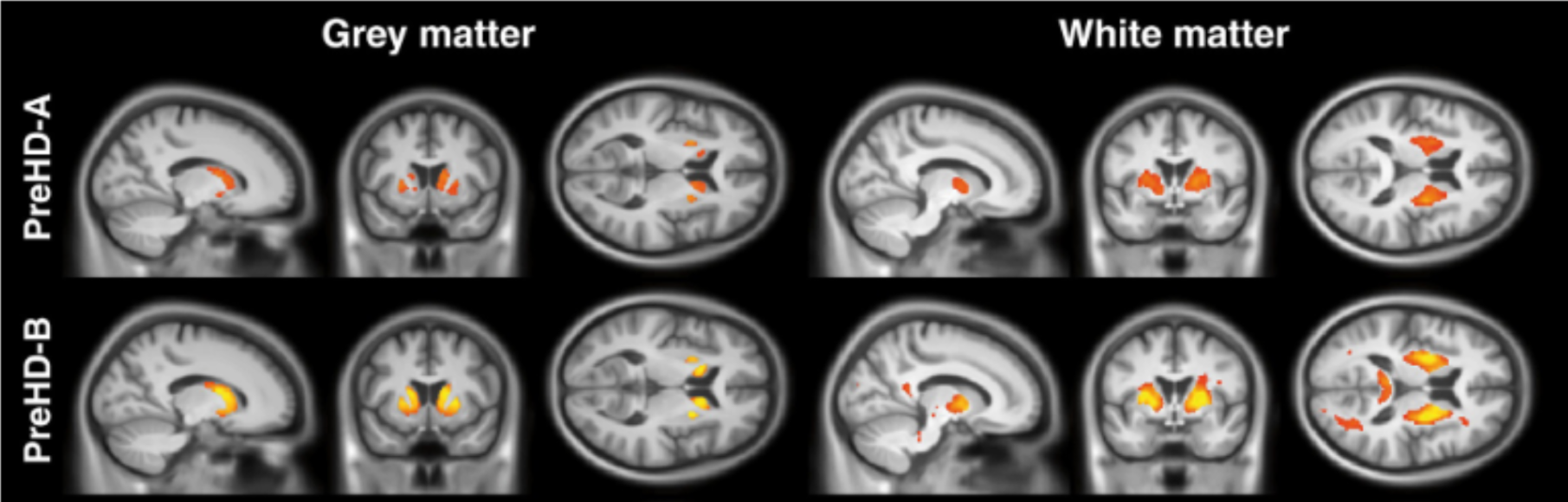
Fig 1. Visualization of brain damage due to Huntington’s disease – red and yellow represent lower and higher damage, respectively. Image from [2].
Challenges in MRI Image Comparisons
MRI measurements serve as essential diagnostic tools for these conditions. Moreover, they offer the potential to identify similarities and differences between individual cases. For instance, when a group of patients responds well to treatment, we can use MRI scans to assess whether a new patient might also respond positively. If the new patient’s MRI resembles those of the positively responding group, it suggests a likelihood of a favorable response to the same treatment.
But how do we compare two MRI images effectively? Simple pixel-by-pixel subtraction isn’t the solution due to variations in measurement conditions and patients’ characteristics, such as head positioning and brain sizes.
Creating a Unique “Fingerprint” for MRI Scans
Instead, we aim to create a unique “fingerprint” for each MRI – a set of distinctive features that characterize the brain comprehensively. These feature lists are known as embeddings. They are easily comparable, as illustrated in Fig. 2. Modern AI solutions can be harnessed to generate such embeddings without explicitly training the models for image differentiation by repurposing pre-trained models. Let’s use image segmentation as an example.
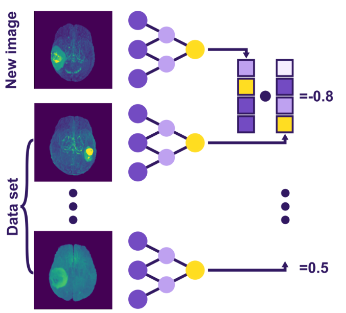
Fig 2. Visualization of the retrieval system – a new image and a previous dataset of images are processed by the same neural network, producing their respective embeddings. These embeddings are then compared, resulting in a quantitative similarity score.
Deep Learning for Image Segmentation
You may be familiar with the dominance of deep learning solutions in image segmentation. That involves identifying important regions – such as tumors – within an image automatically. Deep neural networks excel in this field because they can learn to extract and utilize relevant features for a given task. There are publicly available deep neural networks, one of which is SwinUNETR [3], designed and trained to segment brain tumors in MRI scans. SwinUNETR bears similarities to the architecture known as U-net, with dedicated components for feature extraction and region selection. The central feature, known as the bottleneck feature, is the product of the feature extraction on the left side of the network.
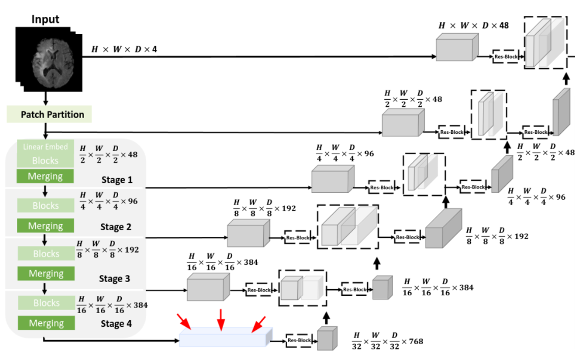
Fig 3. Schematic view of the SwinUNETR neural network. The bottleneck feature is highlighted with red arrows. Image from [3].
Feature Extraction and its Power in Identifying Data Similarities
We can dissect this neural network to extract only the feature extraction part, treating the bottleneck feature as our embedding. In a simplified example, we utilize the BraTS dataset, which was used to train the full SwinUNETR for tumor segmentation.
→ Take a look at our code below the main text.
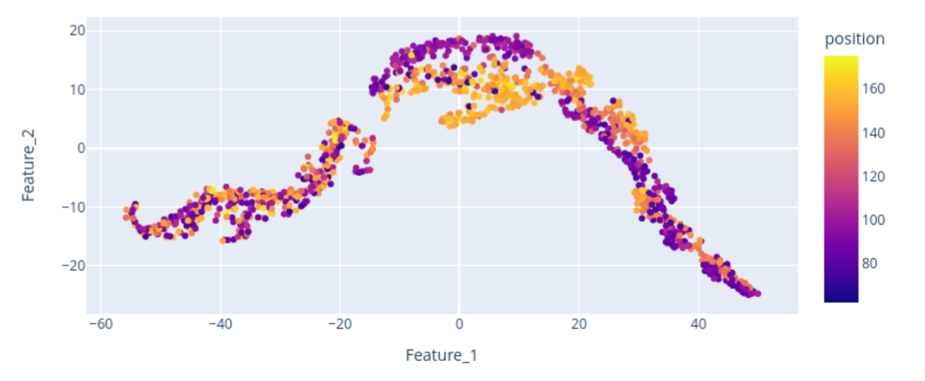
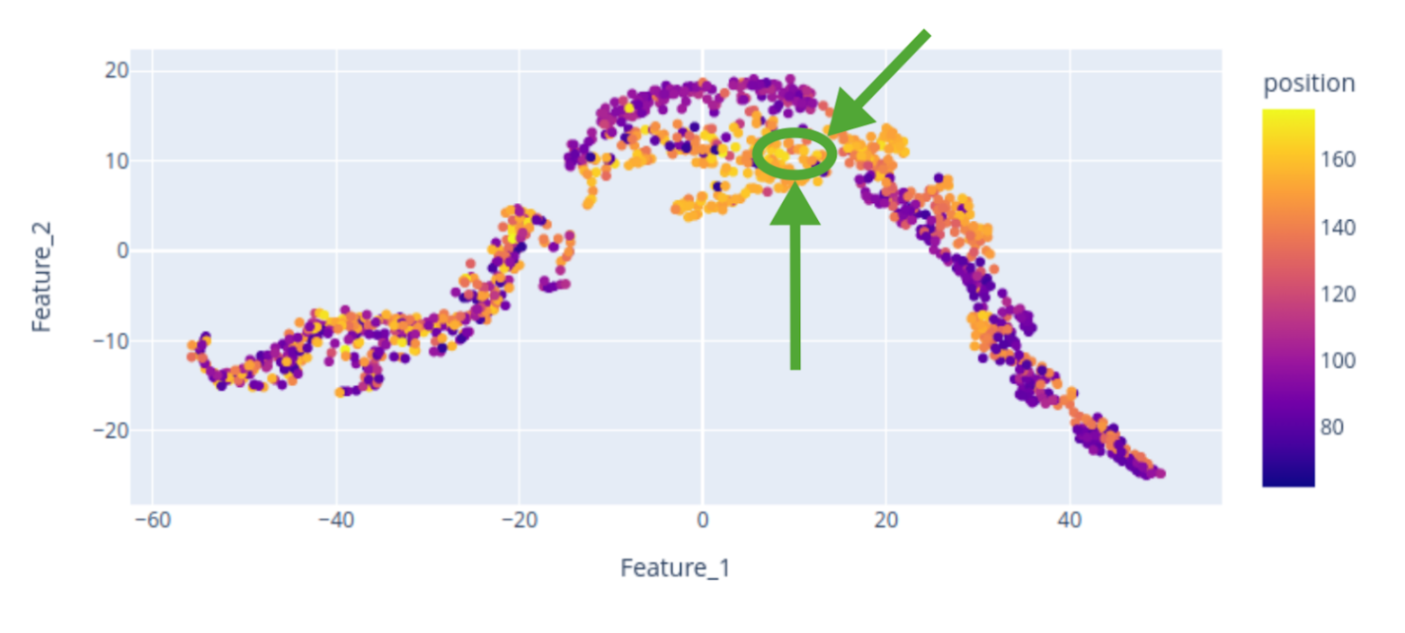
Here, we provide a 2D visualization of the BraTS dataset embeddings, with colors encoding the center of mass of the tumor label along one axis. The center of mass is a representative feature extracted from the tumor labels, demonstrating that the bottleneck feature retains spatial characteristics of the data, including tumor location. The scatterplot reveals that the tumor’s spatial location is encoded in the embedding, although the 2D representation may not perfectly distinguish “right” from “left” tumors. Nevertheless, tumors of the same side tend to cluster together.
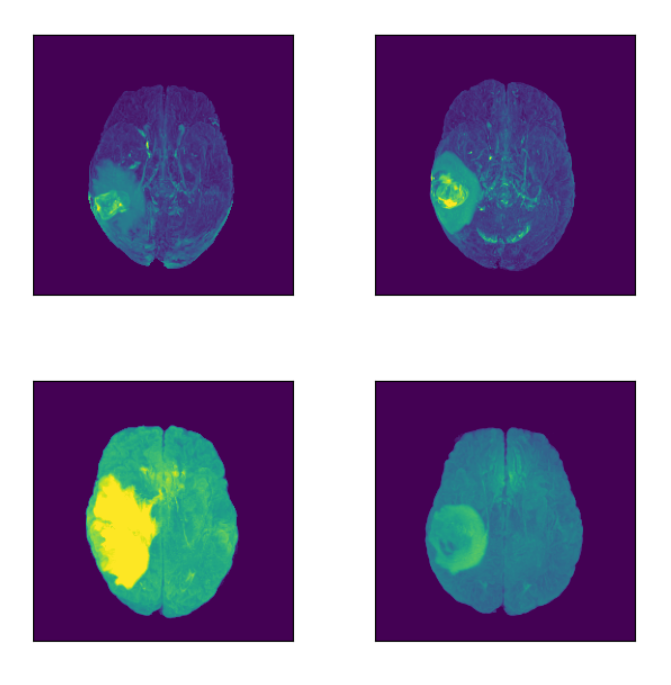
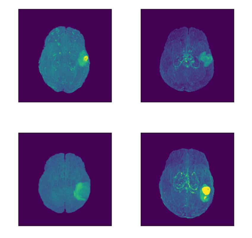
Let’s focus on the highlighted regions (Maximum Intensity Projection of FLAIR modality):
Concluding Insights on MRI Data Retrieval
This illustrative example underscores the power of an effective feature extractor, allowing us to identify dataset similarities and visually verify them. Once we are satisfied with the visual assessment using a scatterplot, we can implement an actual retrieval mechanism. For example, a similarity metric such as the dot product can be employed to find similar cases based on a query example.
In conclusion, AI’s role in modern radiology, particularly in analyzing MRI scans, is undeniably transformative. By integrating advanced AI techniques, we can delve deeper into understanding brain conditions, optimizing patient treatments, and ultimately, paving the way for groundbreaking medical advancements.
Works Cited:
[1] Schwarz, A.J. The Use, Standardization, and Interpretation of Brain Imaging Data in Clinical Trials of Neurodegenerative Disorders. Neurotherapeutics 18, 686–708 (2021). https://doi.org/10.1007/s13311-021-01027-4
[2] Scahill, R. I., Andre, R., Tabrizi, S. J., & Aylward, E. H. (2017). Structural imaging in premanifest and manifest Huntington disease. Handbook of Clinical Neurology, 247–261. doi:10.1016/b978-0-12-801893-4.00020-1
[3] Hatamizadeh, Ali, et al. “Swin unetr: Swin transformers for semantic segmentation of brain tumors in mri images.” International MICCAI Brainlesion Workshop. Cham: Springer International Publishing, 2021., https://github.com/Project-MONAI/research-contributions/tree/main/SwinUNETR/BRATS21
The code used to train SwinUNETR for tumor segmentation:
from monai.networks.nets import SwinUNETR
from monai import transforms
from monai.inferers import sliding_window_inference
import torch
import numpy as np
import pandas as pd
from pathlib import Path
from tqdm import tqdm
roi = 128
batch_size = 1
device = “cuda”
modalities = [“flair”, “t1ce”, “t1”, “t2”]
model = SwinUNETR(
img_size=roi,
in_channels=4,
out_channels=3,
feature_size=48,
drop_rate=0.0,
attn_drop_rate=0.0,
dropout_path_rate=0.0,
use_checkpoint=True,
)
pretrained_pth = “/mnt/Data/SwinUNETR_BraTS_weights/fold0_f48_ep300_4gpu_dice0_8854/model.pt”
model_dict = torch.load(pretrained_pth, map_location=torch.device(device))[“state_dict”]
model.load_state_dict(model_dict)
model = model.to(device)
test_transform = transforms.Compose(
[
transforms.LoadImaged(keys=”image”, image_only=False),
transforms.EnsureChannelFirstd(keys=”image”, channel_dim=”no_channel”),
transforms.NormalizeIntensityd(keys=”image”, nonzero=True, channel_wise=True),
transforms.ToTensord(keys=”image”),
]
)
path_data = Path(“/mnt/Data/SOW2/brats2021_task1/BraTS2021_Training_Data/”)
im_dict_list = [{“image”: [path_data / d.name / f”{d.name}_{m}.nii.gz” for m in modalities]} for d in sorted(path_data.iterdir()) if “BraTS” in d.name]
df = pd.DataFrame([])
for i, im_dict in enumerate(tqdm(im_dict_list)):
x = test_transform([im_dict])
im = x[0][“image”].to(device)
out = sliding_window_inference(im, roi, batch_size, model.swinViT)[4].mean(axis=(2, 3, 4))[0]
out = np.asarray(out.detach().to(“cpu”))
df = pd.concat([df, pd.DataFrame(out).T])
df.to_csv(“/mnt/Data/example/feats_000.csv”)
from scipy.ndimage import center_of_mass
def nii_loader(path):
img_vol = nib.load(path)
return img_vol.get_fdata().T
vols_dir = Path(“/mnt/Data/SOW2/brats2021_task1/BraTS2021_Training_Data/”)
vols_names = [f.name for f in sorted(vols_dir.iterdir()) if “BraTS” in f.name]
vols_labels_paths = [vols_dir / f / f”{f}_seg.nii.gz” for f in vols_names]
vols_centers = [center_of_mass(nii_loader(vol_path)) for vol_path in tqdm(vols_labels_paths)]
vols_centers_array = np.asarray(vols_centers)
df_centers = pd.DataFrame({“Name”: vols_names, “x”: vols_centers_array[:, 2], “y”: vols_centers_array[:, 1], “z”: vols_centers_array[:, 0]})
df_centers.to_csv(“/mnt/Data/example/centers.csv”)
from sklearn.manifold import TSNE
import plotly.express as px
X_embedded = TSNE(n_components=2, learning_rate=’auto’, init=’pca’, perplexity=50).fit_transform(df)
df_embedded = pd.DataFrame(X_embedded, columns=[“Feature_1”, “Feature_2”])
df_embedded[“Name”] = vols_names
df_embedded[“position”] = df_centers[“x”]
fig = px.scatter(df_embedded, x=”Feature_1″, y=”Feature_2″, hover_name=”Name”, color=”position”, width=800, height=400)
fig.show()